Monte Carlo methods is a general term of algorithms that leverage sampling strategies to approximate solution to problems that might be too computationally expensive to solve analytically. The main idea is to use randomness to solve problems that might, in principle, be deterministic.

Monte Carlo methods have been used, for a long time, in several applications in physics-related problems such as Fluid Dynamics, Disordered Materials, Strongly Coupled Solids, Cellular Structures, etc. Other applications include calculations of risk in business and the evaluation of multidimensional definite integrals with complicated boundary conditions. These methods even found a strong foothold on the global carbon emission estimations ante temperature estimation reports of the Intergovernmental Panel on Climate Change (IPCC).

From Monte Carlo Method:

In principle, Monte Carlo methods can be used to solve any problem having a probabilistic interpretation. By the law of large numbers, integrals described by the expected value of some random variable can be approximated by taking the empirical mean (a.k.a. the sample mean) of independent samples of the variable. When the probability distribution of the variable is parametrized, mathematicians often use a Markov chain Monte Carlo (MCMC) sampler. The central idea is to design a judicious Markov chain model with a prescribed stationary probability distribution. That is, in the limit, the samples being generated by the MCMC method will be samples from the desired (target) distribution. By the ergodic theorem, the stationary distribution is approximated by the empirical measures of the random states of the MCMC sampler

In this post we will take a look at some basic Monte Carlo methods with some examples. This might give you an idea of how to use them and which one you might need.

As a matter of disclosure, this post has been compiled from the following sources:

1. Simple MC tutorial
2. MC in practice
3. MC in quantum mechanics
4. MC book
5. Markov Chain MC
6. Monte Carlo Methods (the math)

Example 1: Estimating $\pi$

Monte Carlo methods have different approaches, but tend to follow a particular pattern:

1. Define a domain of possible inputs
2. Generate inputs randomly from a probability distribution over the domain
3. Perform a deterministic computation on the inputs
4. Aggregate the results

For example, consider a quadrant (circular sector) inscribed in a unit square. Given that the ratio of their areas is $\pi/4$ the value of $\pi$ can be approximated using a Monte Carlo method:

1. Draw a square, then inscribe a quadrant within it
2. Uniformly scatter a given number of points over the square
3. Count the number of points inside the quadrant, i.e. having a distance from the origin of less than 1
4. The ratio of the inside-count and the total-sample-count is an estimate of the ratio of the two areas, $\pi/4$. Multiply the result by 4 to estimate $\pi$.

Illustration of point-sampling inside a $1\times 1$ square. The ratio of points inside the circle to the ones outside gives an approximation of $\pi$.

Example 2: Integral approximation

In this example we will try to approximate the following integral

This is an example borrowed from Quantum Mechanics where this integral is used to estimate ground state energies of quantum mechanical systems. There are several approaches to tackle this such as pure Monte Carlo, Variational Monte Carlo, etc.

Let’s start with a pure Monte Carlo approach

Simple Monte Carlo

The simple MC approach is the simplest to understand but the more inacurate. You might remember that we can compute the average value of a continuos function as follows:

In a similar way we can find the average value of an integral by determining the average value of its inegrand $f(x)$. The Monte Carlo technique is built upon this principle: instead of evaluating an indefinite integral, which can sometimes be impossible, let’s instead estimate the average of the integrand and use that to approximate the integral.

the simple MC approach comprises the following steps:

1. Get a random input value from the integration range
2. Evaluate the integrand
3. Repeat Steps 1 and 2 for as long as you like
4. Determine the average of all these samples and multiply by the range

import numpy as np
import math
import seaborn as sns
import random
from matplotlib import pyplot as plt
from IPython.display import clear_output

PI = 3.1415926
e = 2.71828

# lets define a random number generator
def get_rand_number(min_value, max_value):
    """
    This function gets a random number from a uniform distribution between
    the two input values [min_value, max_value] inclusively
    Args:
    - min_value (float)
    - max_value (float)
    Return:
    - Random number between this range (float)
    """
    range = max_value - min_value
    choice = random.uniform(0,1)
    return min_value + range*choice

# lets define our integrand function
def f_of_x(x):
    """
    This is the main function we want to integrate over.
    Args:
    - x (float) : input to function; must be in radians
    Return:
    - output of function f(x) (float)
    """
    return (e**(-1*x))/(1+(x-1)**2)

sns.set_context('talk')
x = np.arange(0, 6., 0.02)
y = f_of_x(x)
fig = plt.figure(figsize=(10,5))
plt.plot(x, y, label=r"$\frac{e^{-x}}{1+(x-1)^2}$", c="tomato")
plt.xlabel("x")
plt.ylabel("y")
plt.legend()
plt.show()

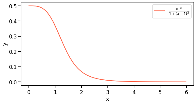
Examplary function to integrate and approximate with Monte Carlo. This function is defined in positive real values and is monotone decreasing.

def crude_monte_carlo(num_samples=5000):
    """
    This function performs the Crude Monte Carlo for our
    specific function f(x) on the range x=0 to x=5.
    Notice that this bound is sufficient because f(x)
    approaches 0 at around PI.
    Args:
    - num_samples (float) : number of samples
    Return:
    - Crude Monte Carlo estimation (float)
    
    """
    lower_bound = 0
    upper_bound = 5
    
    sum_of_samples = 0
    for i in range(num_samples):
        x = get_rand_number(lower_bound, upper_bound)
        sum_of_samples += f_of_x(x)
    
    return (upper_bound - lower_bound) * float(sum_of_samples/num_samples)

crude_mc = crude_monte_carlo(num_samples=10000)
print(f"The crude estimation ofsimple MC approach for the integral is: {crude_mc}")

"The crude estimation ofsimple MC approach for the integral is: 0.7179527733397322"

This results is not so far from the approximation from Wolfram: Wolfram approximation which is: $0.696092$. Now we can try to estimate how confident we are with our estimation. We can quantify the confidence by computing the variance of our estimations. The variance is generally defines as

The variances give us then how much $f(x)$ varies in the domain of $x$. We can then compute the variance as:

def get_crude_MC_variance(num_samples):
    """
    This function returns the variance fo the Crude Monte Carlo.
    Note that the inputed number of samples does not neccissarily
    need to correspond to number of samples used in the Monte
    Carlo Simulation.
    Args:
    - num_samples (int)
    Return:
    - Variance for Crude Monte Carlo approximation of f(x) (float)
    """
    int_max = 5 # this is the max of our integration range
    
    # get the average of squares
    running_total = 0
    for i in range(num_samples):
        x = get_rand_number(0, int_max)
        running_total += f_of_x(x)**2
    sum_of_sqs = running_total*int_max / num_samples
    
    # get square of average
    running_total = 0
    for i in range(num_samples):
        x = get_rand_number(0, int_max)
        running_total = f_of_x(x)
    sq_ave = (int_max*running_total/num_samples)**2
    
    return sum_of_sqs - sq_ave

get_crude_MC_variance(10000)

0.26968839079544155

A variance of $~0.269$ corresponds to an error of $~0.005$. This is not quiet bad but sometimes a lot of precision is required. In the later case a higher number of samples could be chosen, or a bigger range of sampling. But the computation time will increase. In order to tackle this we can also use a little trick caller importance sampling.

Importance sampling

the main idea is that instead of uniformly sampling in the whole range of $x$ we would sample from a distribution of points that are similarly shaped as to the function we want to approximate. This means that we want to improve our estimations of the integral but without increasing the number of samples. To implement this “trick”, we have to find an optimal function that weights the function of interest where the integrand is large. for more details on this please visit the complete webpost or these article Variational Monte Carlo.

Different types of Monte Carlo Simulations

1. Plain Monte Carlo: Simple sampling approach of a high dimensional space
2. Markov Chain Monte Carlo: A method for sampling high dimensional data. Most of these methods create an ensemble
3. of random walkers that start from a set of random positions that are reasonably separated and then on each iteration try to move to a point where the integral is thought to be high. Tend to perform better than plain MC in spaces of high number of dimensions. More details can be found on the definitions of specific methods: Metropolis-Hashtings, Gibbs sampling, Hamiltonian Monte Carlo, etc.
4. Sequential Monte Carlo: Used to estimate the internal state of dynamic systems when partial measurements are made.
5. Quasi Monte Carlo: Uses quasi-random sequences instead of the traditional pseudo-random sequences. This leads to a faster convergence $O(1/N)$ compared to plain Monte Carlo $O(N^{-1/2})$ etc. etc.

x = np.arange(100)
y1 = 1/x
y2 = x**(-0.5)
plt.figure(figsize=(20,5))
plt.plot(x, y1, label="Quasi Monte Carlo", c="tomato")
plt.plot(x, y2, label="Monte Carlo", c="royalblue")
plt.title("Convergence rate")
plt.legend()
plt.show()

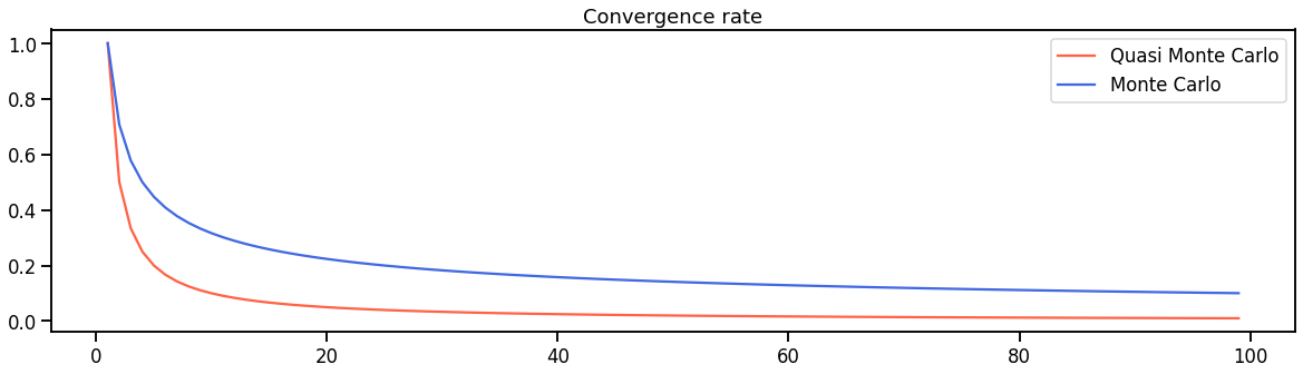
Exemplary convergence rate for pure Monte Carlo and Quasi Monte Carlo approximations.

Example 3. Light transport in tissue

Sampling random variables

Consider a random variable $\chi$. In this case it represents the step size of a photon when it propagates in a medium, or the angle of deflection of the photon when it interacts with a particle in tissue (scattering). Lets now consider the probability density function in an interval $(a,b)$ that is normalized as follows:

In order to simulate the propagation of a photon in tissue we wish to sample values of $\chi$ using a pseudo-random number generator. A computer can generate a random variable $\xi$ which is uniformly distributed over the interval $(0,1)$. Then, the cummulative distribution function of this uniformly distributed random variable is:

To sample a non-uniformly distributed function, we assume that there is a non-decreasing function $f$ that maps $\xi\in (0,1)$ to $\chi\in(a,b)$. That is $\chi =f(\xi)$, therefore, both variables have a one-to-one mapping. This leads to the following (complete deduction here):

Photon step size

We sample from the probability distribution of the photon’s free path $s\in[0,\infty)$. The probability of interaction per unit path length in the interval $(s’, s’ + ds’)$ is:

where $\mu_t = \mu_a + \mu_s$ is the total scattering coefficient

We can integrate this in the interval $(0,s_1)$ which leads to an exponential distribution, where $P{ s\geq 0} = 1$ is used:

Which we can then integrate:

This can then be used to choose a step size:

Photon scattering

The probability distribution for the cosine of the deflection angle during scattering events is described by the scattering function that Greenstein proposed on 1994:

where $\theta \in [0, \pi)$ is the scattered angle, $g = <\cos\theta>$ is the anisotropy of the tissue and has a value between -1 and 1. $g=0$ means isotropic scattering and $g=1$ means forward scattering. The choice of $\cos \theta$ can now be interpreted using a random number $\xi$:

fig, ax = plt.subplots()
x = np.arange(0, 2*np.pi, 0.01)
g = 0.2
y = (1-g**2) / (2*(1+g**2 -2*g*np.cos(x))**(3/2))
plt.plot(x,y, label=r"$p(\theta)$", c="tomato")
plt.legend()
plt.show()

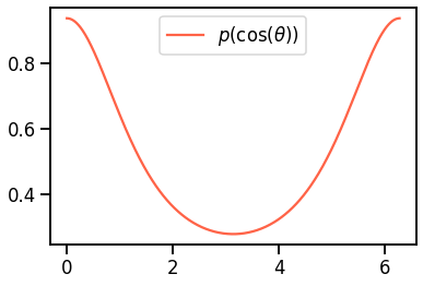
Probability distribution as a function of the cosine of $\theta$.

n_iter = 200
pos_x = [0]
pos_y = [0]
mu = 0.9
g = 0.1
for i in range(n_iter):
  s1 = -np.log(np.random.rand()) / mu
  cos_tetha = (1/(2*g)) * (1 + g**2 - ((1-g**2)/(1-g+2*g*np.random.rand())**2))
  new_x = pos_x[-1] +  s1 * cos_tetha
  new_y = pos_y[-1] + s1 * np.sin(np.arccos(cos_tetha))
  pos_x.append(new_x)
  pos_y.append(new_y)

fig, ax = plt.subplots()
plt.plot(pos_x, pos_y, lw=2, c="tomato")
ax.set_ylim(120, 0)
plt.title("Pothon path")
plt.show()

Exemplary photon path in tissue media. Notice that most of the scattering effects tend to disperse the photon in a downward direction. This is due to the distribution of $p(\cos(\theta))$.

from matplotlib.collections import LineCollection

fig, ax = plt.subplots()

steps = np.arange(100)[::-1]
points = np.array([np.array(pos_x), np.array(pos_y)]).T.reshape(-1, 1, 2)
segments = np.concatenate([points[:-1], points[1:]], axis=1)
# Create a continuous norm to map from data points to colors
norm = plt.Normalize(steps.min(), steps.max())
lc = LineCollection(segments, cmap='viridis', norm=norm)

# Set the values used for colormapping
lc.set_array(steps)
lc.set_linewidth(2)
line = ax.add_collection(lc)
fig.colorbar(line, ax=ax)
plt.autoscale()
ax.set_ylim(120, 0)
plt.title("Pothon path")
plt.show()

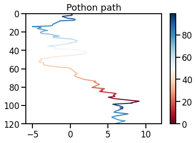
Illustration of photon path in tissue. The colors represent the depth within the tissue sample.

fig, ax = plt.subplots()
for j in range(10):
  n_iter = 200
  pos_x = [0]
  pos_y = [0]
  mu = 0.9
  g = 0.1
  for i in range(n_iter):
    s1 = -np.log(np.random.rand()) / mu
    cos_tetha = (1/(2*g)) * (1 + g**2 - ((1-g**2)/(1-g+2*g*np.random.rand())**2))
    new_x = pos_x[-1] +  s1 * cos_tetha
    new_y = pos_y[-1] + s1 * np.sin(np.arccos(cos_tetha))
    pos_x.append(new_x)
    pos_y.append(new_y)
  plt.plot(pos_x, pos_y, lw=2)
plt.title("Pothon path")
ax.set_ylim(120, 0)
plt.show()

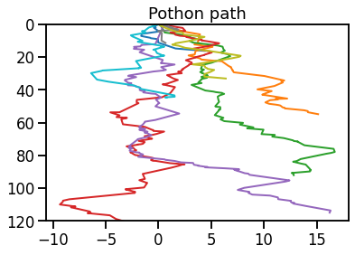
Photon paths computed with Monte Carlo over several runs.

If we then simulate many photons, we can create a heatmat with the distribution of paths that the photons take inside the media, as depicted in the animation.

Photon path distribution after simulating multiple photon trajectories

Conclusions

We have explored several examples of where Monte Carlo approximations are used. Several of the code examples shown here are not optimized for run-time, so any attempts to re-use this code should consider also different strategies for optimization, e.g. parallelization using a GPU. One library that has seen a lot of development in the last years that could help many people run Monte Carlo simulations for photon transport in biological tissue is SIMPA, a Python tool that allows to interact easily with MCX.