

The purpose of this post is to summarize different techniques used in the design of physics-informed neural networks (PINNs). Although advanced topics in Machine Learning and physics are discussed in this post, it is not an in-depth tutorial on everything there is to know about PINNs. It is expected that you have a basic understanding of both Machine Learning and physics.
The mathematical notation in this post might not be consistent across sections. For example, the symbol $u$ might be used to refer to fluid velocity in one section, and to refer to a generic variable in other sections.
PINN categories
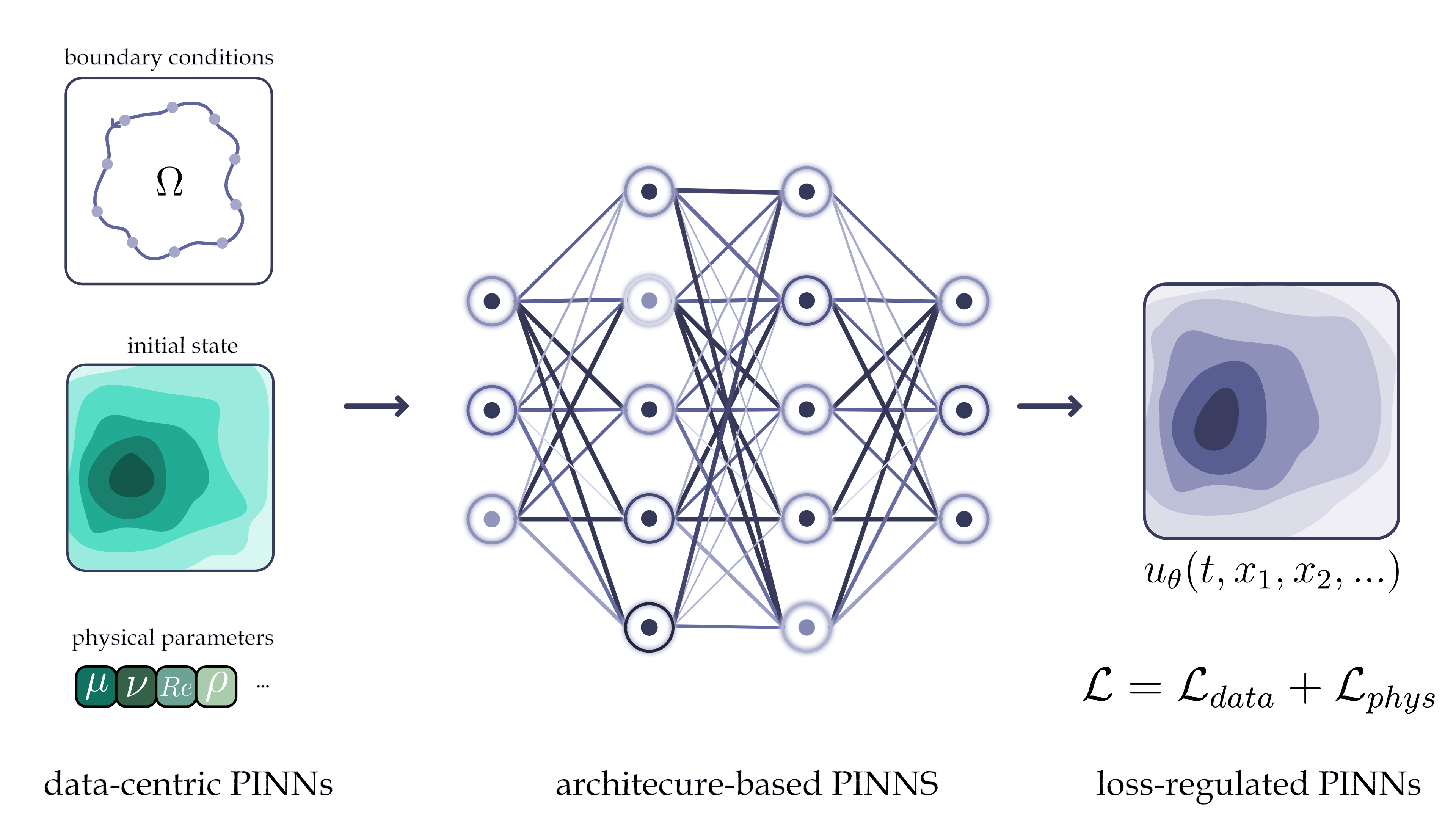
At the time of writing this post, there are three main categories of PINNs depending on which aspects of the training pipeline are “informed” by physics information. Those categories are: data-centric, architecture-based, and loss-regulated PINNs. The image below illustrates which parts of the pipeline each category addresses. Usually, a PINN will accept some input, in any form or shape possible, and output a physical or “physical-related” property $u$, which is parametrized by the network parameters $\theta$. The reason I mention that PINNs can output “physical-related” properties is that we might be interested in generating a quantity that we later on transform into a physical property. For example, a PINN can be used to calculate a material’s porosity, which in turn can be used to calculate the material’s thermal conductivity.
Data-centric PINNs
This category of PINNs is easily identified by its heavy use of data that has been generated by a simulator or collected via experimentation. At its core, data-centric PINNs aim to reproduce the distribution of the physics-generated data that they have seen during training, with the hope that they will generalize to unseen data.
The main advantage of this approach is that, assuming a simulator exists or that experiments are feasible, the training procedure of a PINN is straightforward because all traditional training pipelines can be used.
The biggest shortcoming of this approach is that there is no physical guarantee on the output of the network. This means that the output of the network can theoretically be any quantity, even if it is not physically plausible. An example of this is a network that generates a negative density in a particular region of fluid volume. Although there are ways to mitigate such mistakes, for example by applying a threshold to the output, there are other physical law violations that cannot be corrected by such simple techniques, e.g. conservation of mass and energy.
Loss-regulated PINNs
The main objective of a PINN is to generate outputs that are in line with what physics laws demand. To mitigate physical violations of the network outputs, custom losses are used during training. By far, the most common type of loss found in PINNs are partial differential equation residuals (PDE-residual). A PDE-residual loss measures how badly the neural network outputs violate a known physical law. Any given PDE has a corresponding residual, which is simply obtained by moving all terms to one side of the equality, so that the residual is zero when the PDE is satisfied exactly. For example, suppose a PINN estimates temperature $T_\theta (x,t)$; the governing equation is:
\[\frac{\partial T}{\partial t} = \alpha \frac{\partial^2T}{\partial x^2},\]where $\alpha$ is the thermal diffusivity. The PDE-residual is then:
\[\mathcal{R}(x,t) = \frac{\partial T_\theta}{\partial t} - \alpha \frac{\partial^2T_\theta}{\partial x^2},\]and the loss becomes:
\[\text{L}_{PDE} = \frac{1}{N}\sum^N_{i=1}|\mathcal{R}(x_i,t_i)|^2,\]where $N$ is the number of points. This ensures that the network not only reproduces the data that is being fed, but that the outputs satisfy the governing physical laws that the problem demands. Similar residuals and losses can be found across many other applications.
Architecture-based PINNs
This is one of the less developed categories of PINNs, potentially because the other two categories are the ones that have the largest influence in most practical applications. Interpreting “architectural changes” loosely, the architectural changes that dominate in PINNs are the following.
-
Output structure: The core idea here is to train a network to predict a more generic property that is then transformed to represent some physical property, or to enforce boundary conditions. For example, if a network is meant to estimate a physical property $u$ under the boundary conditions:
\[u(0) = 0, \quad u(1)=1\]Instead of having the network estimate $u(x)$, one can instead predict another property $\mathcal{U}_\theta (x)$ which can then be transformed into:
\[u(x) = x + x(1-x)\mathcal{U}_\theta (x)\]Notice how this transformation enforces the boundary conditions on $u(x)$ without having to worry about what the network outputs. Another concrete example can be found in fluid dynamics, where for an incompressible flow, rather than estimating velocity components $u, v$, the network can predict $\mathcal{U}_\theta (x, y)$ and then define:
\[u =\frac{\partial \mathcal{U}_\theta}{\partial y}, \quad v = -\frac{\partial \mathcal{U}_\theta}{\partial x}\]This naturally incorporates the physics through the relationship of the network output and the physical variables $u, v$.
-
Fourier embeddings: Plain MLPs are known for being lazy at learning details (high frequencies). They learn the broad smooth shape of a solution quickly, but they learn fast changes slowly. This is also known as “spectral bias”. This is particularly important in PINNs because the physical equations that they have to solve usually care a lot about how fast things change. For example, in fluid dynamics, a sudden change in pressure can have a large influence on the final desired output. The solution is to transform the inputs by embedding them into Fourier features (set of cosine and sine functions):
\[\gamma(x) = [\cos(2\pi Bx), \sin(2\pi Bx)],\]where $B$ is a matrix of frequencies, usually sampled from $B_{i,j} \sim \mathcal{N}(0, \sigma^2)$. One more intuitive way to think about this transformation is that instead of forcing the MLP to learn all frequencies (high and low), it receives a set of generated signals that the network has to learn to combine to generate the desired output. This is similar to how combining stencils can produce much more complicated illustrations that would be difficult to generate by hand.
A variation of this approach uses multiple $B$ matrices to provide the network with multi-scale embeddings. In some applications this has proven to perform better than using a single scale.
-
Modified MLP gating architecture: PINNs suffer from two distinct gradient pathologies, and it is worth keeping them apart. The first is an imbalance between loss terms: the gradient updates coming from PDE-residuals, boundary/initial-condition terms, etc. are badly mismatched in magnitude, so the PDE-residual gradient can drown out the gradients from the boundary conditions, or the other way around, which leads to non-convergence or convergence to the wrong minimum. That one is not an architectural problem and is addressed by adaptive loss weighting (learning-rate annealing, NTK-based weights, self-adaptive weights). The second is gradient flow through depth: the input signal and the gradients that carry it have to survive every layer of the network, and in deep plain MLPs they degrade along the way. This is the one the modified MLP targets, by introducing a gating mechanism with a similar idea as skip connections. While plain MLPs just stack layers as:
\[H^{(k+1)} = a(W^{(k)}H^{(k)} + b^{(k)}),\]where $a$ is the activation function, the modified MLP adds two “encoder” transformations of the input that are computed once and then injected into every layer as follows. Given an input $x$, one can compute two transformations $U$ and $V$:
\[U = a(W_ux+b_u), \quad V=a(W_vx+b_v),\]and for the first layer:
\[H^{(1)} = a(W^{(1)}x+b^{(1)}),\]then for each hidden layer $k$:
\[Z^{(k)} = a(W^{(k)}H^{(k)}+b^{(k)})\] \[H^{(k+1)} = (1-Z^{(k)}) \odot U + Z^{(k)} \odot V\]Because $U$ and $V$ are computed from the input, and they are fed directly into each hidden layer, information about $x$ does not have to survive the entire trip, but it can use this “highway” path. This is a similar idea that is found in skip connections: keep the gradients flowing through the entire network and provide a way for gradients to travel all the way. This architecture has been shown to provide empirical robustness across different applications.
Fourier embeddings and modified MLP gating architecture are usually used as complements because they address two main challenges: which frequencies can be represented by the network, and whether the network can reach a “good” solution.
Non-dimensionalization
Non-dimensionalization in the context of PINNs refers to rescaling the governing equations, inputs, and outputs so that all quantities become dimensionless and, ideally, of order $O(1)$. This is already something often done in many fields of physics. A concrete example of this is the Reynolds number in fluid dynamics, where the value of this number is a characteristic of the type of flow (laminar vs. turbulent). For PINNs, non-dimensionalization is sometimes the difference between a network that converges and one that doesn’t.
Non-dimensionalization becomes particularly relevant in PINNs because physical properties often live on completely different scales. Spatial coordinates might live in $[0, 10]\,\text{cm}$, while time might be in $[0, 1200]\,\text{s}$, and temperature in $[300, 1200]\,\text{K}$. This is a known issue in Machine Learning, where gradients along such dimensions often drown out the rest due to the scale disparity. The recipe to address this is the following:
- Choose characteristic scales (length, time, velocity, temperature, etc.).
- Define dimensionless variables, substitute them into the PDE, and collect the resulting dimensionless groups (Reynolds number, Péclet number, etc.).
- Train the network on the new variables and convert them back at the end.
Concrete example: Heat equation Consider a rod of length $\ell=0.1\,\text{m}$, diffusivity $\alpha=1\times10^{-5}\,\text{m}^2/\,\text{s}$, and temperature in the range of $[300, 400]\,\text{K}$. The diffusion PDE is given by:
\[\frac{\partial T}{\partial t} = \alpha \frac{\partial^2T}{\partial x^2}\]By defining the dimensionless variables $x^* =x/\ell$, $t^* =\alpha t/\ell^2$ (diffusive time scale) and $T^* =(T-300)/100$, the PDE is rewritten as:
\[\frac{\partial T^*}{\partial t^*} = \frac{\partial^2T^*}{\partial {x^*}^{2}}\]Now the dimensionless variables are in ranges that can be handled much better by a network: $x^* \in [0, 1]$ and $T^* \in [0,1]$, while the coefficient $\alpha$ has disappeared entirely.
Practical aspects: In practice, PINNs do not just see one sample as in the previous example, they see thousands or millions of samples with different physical scales. The question here is which “typical” dimensional properties (length, time, etc.) should be chosen to create the non-dimensional variants. The answer is not straightforward; one can do this per sample independently, or based on aggregated statistics over an entire dataset. Both have advantages and disadvantages; often the decisive factor is whether the different scales carry information that is interesting for the problem at hand. For example, does it matter if the temperature is different across scales? Or is that something that can be ignored?
Non-dimensionalization vs standard ML normalization
Non-dimensionalization often sounds very similar to other common normalization techniques in ML (z-score: $x^* = (x-\mu)/\sigma$). The main difference is that z-score normalization is empirical and blind to meaning, while the dimensionless properties carry the meaning of the physical problem (e.g. Reynolds number). Non-dimensionalization also changes the entire set of equations; this includes the loss function, while z-score normalization only re-scales the inputs/targets.
Even more, standard z-score normalization treats each feature independently; each feature gets its own mean and standard deviation. In contrast, non-dimensionalization naturally couples features because the physical equations tie them together. Think about how a change in length scale naturally introduces a change in velocity scale. This coupling is entirely lost in traditional ML normalization approaches.
The table below highlights the main differences between both approaches.
| ML normalization | Non-dimensionalization | |
|---|---|---|
| Source of scales | Dataset statistics ($\mu$, $\sigma$) | Governing equation + geometry |
| Requires data? | Yes | No (works for pure forward problems) |
| What it changes | Inputs/targets only | The equation and its residual |
| Axes | Independent per feature | Often coupled by the physics |
| Interpretability | Scales are just numbers | Scales are physical, groups are meaningful |
Conservation laws in PINNs
This is perhaps one of the most challenging aspects of PINNs because the output of an ML model tends to be unpredictable and unbounded (regression tasks). If a PDE-residual loss is already present in the loss terms, this often tends to enforce conservation laws because they are often embedded within such PDEs, for example the conservation of mass can be written as: $\partial \rho/\partial t + \nabla \cdot(\rho u) = 0$. Another way to enforce global conservation laws is to introduce additional penalties on the loss that take into account the property that should be conserved. For example, if it is important that the total amount of mass in a volume remains constant, the integral of the density estimated by a network $\rho_\theta(x,t)$, parametrized by the model parameters $\theta$, can be used to regularize the loss:
\[\text{L}_{const} = \left| \int_\Omega \rho_\theta(x,t) d^3x - M_0 \right|^2,\]where $\Omega$ is the spatial domain, and $M_0$ is the total initial mass. Both of these approaches only aim to force the network to estimate properties that are close to a physically correct solution. Both of them do not enforce an exact solution where conservation laws are guaranteed. Luckily, there are other interesting approaches that can be used to try to make the conservation laws in PINNs a guarantee by design. Such approaches are discussed in the following sections.
Error correction
One of the simplest ways to ensure conservation laws relies on the assumption that the solution provided by a PINN is close to a perfect solution. Under such assumption, the network output can be transformed by approximating it to the closest solution for which the conservation laws are exact. For example, in the case that the conservation of mass is a must in an incompressible flow, it is reduced to: $\nabla \cdot u = 0$, where the corrected velocity field is defined by:
\[u_{corr} = u_\theta + \delta u \quad\text{s.t.}\quad \nabla \cdot u_{corr}=0\]A standard way to find such correction term is to find the closest divergence-free velocity field:
\[u_{corr} = \mathop{arg\,min}_v \| v - u_\theta \|^2 \quad\text{s.t.}\quad \nabla \cdot v = 0,\]to solve this minimization problem, a Lagrange multiplier field $\lambda$ is introduced to enforce the divergence-free constraint. Stationarity of the resulting Lagrangian with respect to $v$ forces the correction to be a pure gradient, $\delta u = -\nabla \lambda$, so the corrected velocity field becomes:
\[u_{corr} = u_\theta - \nabla \lambda,\]where $\lambda$ is chosen such that:
\[\nabla \cdot u_{corr} = 0,\]therefore this constraint becomes:
\[\nabla \cdot (u_\theta - \nabla \lambda) = 0,\]which gives rise to the Poisson equation:
\[\nabla^2\lambda = \nabla \cdot u_\theta\]The problem of finding the closest solution to $u_\theta$ that ensures mass conservation becomes solving the Poisson equation for $\lambda$ and computing from it $u_{corr} = u_\theta -\nabla \lambda$. Notice that this equation has non-unique solutions unless boundary conditions are considered.
Notice that this specific transformation is applicable only to divergence-free constrained problems. For other applications and conservation laws, the exact formulation certainly must change.
Physical state guarantees
Structuring a PINN such that the output is guaranteed to respect a physical law is one of the cleanest ways to enforce physics in ML. At its core, the main concept is to interpret the output of a network as what is known in physics as a “potential”, which can then be used to derive the physical property of interest. In this way, conservation laws become an algebraic identity that is impossible for the network to violate.
As an example, consider once more the incompressible fluid flow, where the mass conservation law requires that $\nabla \cdot u = 0$. Instead of directly interpreting the network output as the velocity field, it can be interpreted as the vector potential $A$ (3D), which corresponds to a “potential” function from which the velocity field $u$ can be derived as follows:
\[u = \nabla \times A\]Because the fundamental property of the curl operator is that $\nabla \cdot (\nabla \times A) \equiv 0$, the conservation of mass is mathematically guaranteed when the network output is interpreted as $A$.
Similarly, other formulations can be found across applications, although not always obvious: Dirichlet boundary conditions, periodicity conditions, electrostatic fields being irrotational, positivity, exact normalization, antisymmetric nature of electronic wave functions, etc.
Symmetry invariance
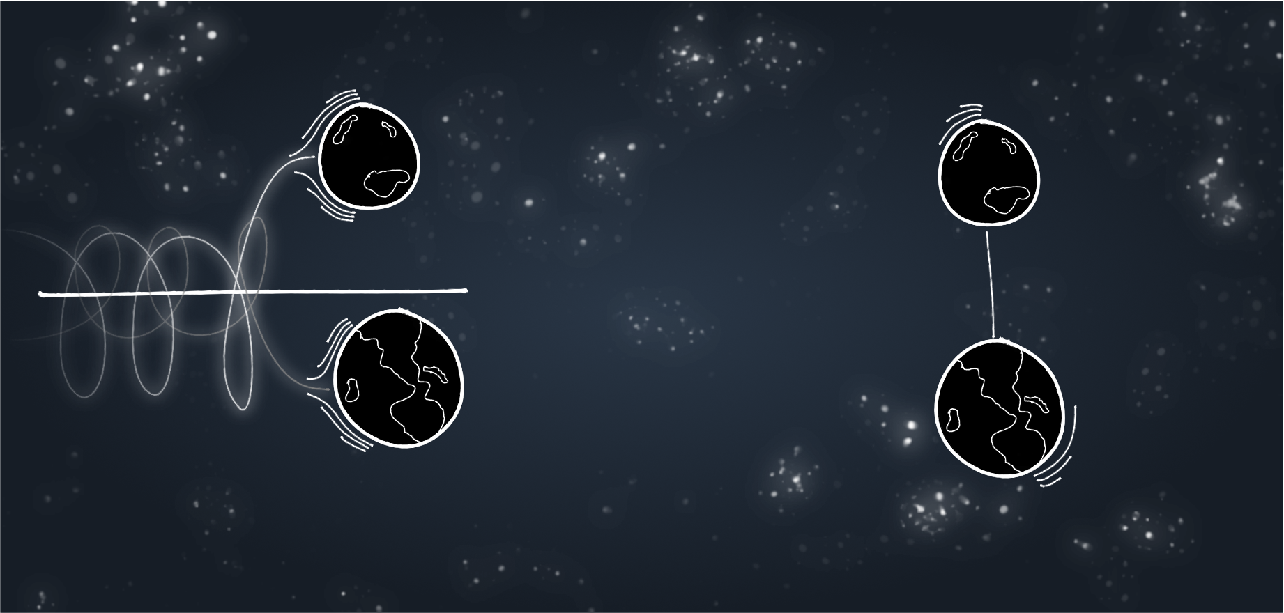
Symmetry is a very interesting aspect in physics. It often allows to simplify problems dramatically, like the two-body gravitation problem. This problem has six coordinates (three per object), but it can be reduced to one radial coordinate due to the rotational and translational symmetries of the problem as well as due to conservation of the angular momentum. An even more interesting aspect of symmetries in physics is related to Noether’s theorem:
If a system has a continuous symmetry property, then there are corresponding quantities whose values are conserved in time
– Noether’s theorem
This has ramifications for PINNs, but it is worth being precise about what Noether’s theorem actually buys. The theorem applies to a continuous symmetry of the action, so it only hands over a conserved quantity when the network parametrizes the object the action is built from: the Lagrangian or the Hamiltonian, as in Lagrangian and Hamiltonian neural networks. There, a symmetry of the learned Lagrangian translates directly into a quantity that the resulting dynamics conserve exactly.
A network that merely maps coordinates to a solution is a different situation. Making such a network invariant is still useful, but as an ansatz rather than as a Noether mechanism: it restricts the hypothesis space to functions that already respect the symmetry, which removes a whole class of wrong solutions and makes the remaining fit easier. The easiest way to do this is to transform the inputs, so instead of feeding raw coordinates like $(x)$, the magnitude could be fed $r=|| x ||$, which makes the network’s output rotation-invariant by construction. That alone conserves nothing; getting an exactly conserved quantity out of it takes the extra step shown at the end of this section, where the conserved value is built into the output parametrization itself.
Another way is to use layers that have some equivariance properties, like group-equivariant CNNs, or E(3)/SE(3)-equivariant networks (Tensor Field Networks, e3nn) for 3D rotation/translation/reflection. Notice that equivariance is not the same as invariance, and equivariance alone does not guarantee that a physical property will be conserved. It is, however, a key ingredient that leads to the kind of invariance that Noether’s theorem requires to guarantee the conservation of a physical property. An invariant scalar energy $E$ gives equivariant forces automatically via $F = -\nabla E$. Equivariance is then a necessary condition, not a mechanism that produces invariance.
To make this more concrete, consider the problem of a particle in a central potential (planetary orbit). Here the motion equations are governed by:
\[m\frac{d^2x}{dt^2} = -\nabla E(\|x\|),\]where the potential depends only on the magnitude of $x$, which indicates a rotational invariance. By Noether’s theorem, this leads to the conservation of a property, in this case the angular momentum $L$. In the naive approach, a PINN could receive as input $(x(t), y(t))$, and it would attempt to minimize the residual. This would approximate the solution and potentially attempt to make changes in the angular momentum more difficult. This would however not guarantee conservation of the angular momentum. It would merely be an approximation that will likely drift over time.
The invariant approach would exploit the rotational symmetry by working in polar coordinates $(r, \phi)$. This allows one to parametrize a network to output only $r(t)$ and only generate $\phi(t)$ by processing $r(t)$. A hard constraint can then be imposed on the angular momentum $L_0 = mr^2(t) \frac{d \phi}{d t} = \text{constant}$ by getting $r(t)$ from the network output and integrating $\frac{d \phi}{d t} = L_0 /(mr^2(t))$ to get $\phi$:
\[\phi(t) = \phi_0 + \int_0^t \frac{d \phi}{d s} ds = \phi_0 + \int_0^t \frac{L_0}{mr^2(s)}ds\]Because the network only outputs $r(t)$, and $\phi(t)$ is only computed from that output, the conservation of angular momentum is a mathematical guarantee.
Time domain PINNs
PINNs that aim to estimate the time evolution of physical properties (trajectories) differentiate themselves from other PINNs due to the main property that arises from the time domain: causality. Causality in this context means that the physical state of a system at a later time depends on the state at an earlier time. A naive implementation would treat time as one more input parameter, and have the network output the entire system state at that time point. This has been empirically proven to be very difficult to converge due to causality violation: the residual is minimized over all $t$ simultaneously, so the network can fit late times before the early solution is resolved, converging to a wrong branch.
Other methods take a more physics-related approach by generating time steps one at a time, where each new time step becomes the input of the network. These are also known as autoregressive models. This keeps the causality intact at the cost of more compute, since parallel training of all time steps is not possible. This is also by far the most common approach that is found in time-domain PINNs. Something that is worth considering in this approach is how the loss is computed and back propagated. There are two approaches: pass as input the previous network output, compute the loss and accumulate it over steps (rolling loss), or pass as input the ground truth history, compute the final loss in the last step and back propagate only the last one. The main differences in these two approaches are that one of them allows the network to learn from its previous mistake (rolling loss), while the other predicts the next steps assuming all previous ones are correct.
The approach followed by discrete-time PINNs is a clever twist on physics-informed neural networks that split the labor between old and new tools. Rather than asking a neural network to learn how a system evolves over time, the usual approach, which struggles with fast changes and long time spans, they hand the time-stepping over to a battle-tested classical method (a high-order implicit Runge-Kutta integrator) and let the network handle only the spatial dependence. Given a spatial coordinate, the network outputs the $q$ internal “stages” of the integrator plus the solution at the next time level, all as functions of space alone; time never enters as an input. The neat part is that by having the network juggle all of those stages at once, you can crank the accuracy up to levels that would be hopelessly expensive with traditional solvers, letting you leap forward in time in a single enormous, rock-stable step. In the original demonstration, this let the method jump across a big chunk of time in one go while still sharply capturing a shockwave, combining the reliability of classical numerical methods with the flexibility of neural networks.
Putting it all together
The techniques covered here are not competing alternatives but complementary layers, each addressing a different failure mode. The starting point is where physics enters the pipeline: data-centric PINNs lean on a physics-based simulator (or experimental data) and reuse standard training pipelines, but offer no guarantee that outputs are physically plausible; loss-regulated PINNs add PDE-residual terms that penalize violations of the governing equations; and architecture-based PINNs bake the physics into the network itself through output transformations that enforce boundary conditions, Fourier embeddings that counter spectral bias, and modified MLP gating that keeps the input signal and its gradients alive through depth. In a real project these stack on top of each other: a data loss anchors the solution, a PDE-residual enforces the equations, adaptive loss weights keep the residual and boundary terms from drowning each other out, Fourier features let the network represent sharp changes, and the gating architecture helps it actually reach a good minimum.
Two further ingredients cut across all of the above. Non-dimensionalization usually comes first: rescaling the equations, inputs, and outputs to be of order $O(1)$ so that gradients along wildly different physical scales do not drown each other out. Unlike blind z-score normalization, it rewrites the residual itself and couples variables the way the physics does. Conservation laws then sit on a spectrum from soft to hard: penalty terms and integral constraints only nudge the network toward admissible solutions, error correction projects the output onto the nearest solution that satisfies the law exactly, and potential-based or symmetry-based formulations turn the law into an algebraic identity the network cannot violate. Finally, when the problem is a trajectory in time, causality pushes toward autoregressive rollouts and a choice between a rolling loss that lets the network learn from its own mistakes and a last-step loss that assumes a perfect history. The overall guideline is to pick the weakest mechanism that still guarantees what the problem genuinely requires, and layer the cheaper approximate techniques around it.